Introduction
It’s been a few month since I started pondering making a better ocean for Cosmos Journeyer’s procedural planets. To have actual waves moving around and not just a scrolling normal maps would make a significant difference in visual quality.
Coincidentally, I was also taking a course on computer animation (INF585) at Ecole Polytechnique, and I had the opportunity to choose my final project. Long story short, I decided to implement Jerry Tessendorf’s FFT-based ocean simulation on WebGPU, and this is my project report.
I came across many different techniques to simulate an ocean during my investigation, but I was definitely seduced by the realism of the FFT ocean simulation, and the fact that it is actually real-time.
I was also inspired by existing work on the subject by Popov72 and Acerola that made the math behind the ocean simulation less intimidating.
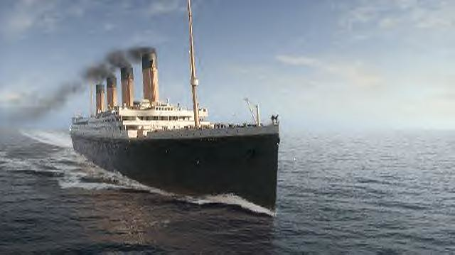
FFT-based ocean simulations are quite popular and you came across one if you ever watched Titanic:
With Cosmos Journeyer being implemented using Typescript and BabylonJS, I decided to use them as well for this project with the intent of integrating the ocean simulation into the game in the near future. The entire project is available on GitHub under an MIT license, you can find a link at the end of this post.
Here is a video of what you can expect from the final result:
Theoretical Background
The main idea behind the FFT ocean simulation is that the ocean surface can be represented as a sum of sinusoidal waves. Not just 10 or 20 waves, but thousands of them! Of course we are not going to sum them all by hand, that would be very slow even inside a vertex shader.
The solution is to use an Inverse Fourier Transform: from a given complex wave spectrum that specifies the amplitude and phase of waves in all directions, we can directly compute the sum of sinusoidal waves without having to compute each wave individually.
The Inverse Fourier Transform by itself is a costly operation, and it would still be too slow if it were not for the Fast Fourier Transform (FFT) algorithm. The FFT algorithm is a clever way to compute the Fourier Transform in O(n log n) time complexity instead of O(n^2).
So the pipeline is as follows:
Generate a wave spectrum using some statistical model
Compute the inverse FFT of the wave spectrum to get the height of the waves at each point in space
Translate the ocean vertices vertically using a vertex shader
Make a realistic shader to make it look like actual water
Generating the Wave Spectrum
Okay, so we need a wave spectrum: a representation of the amplitude and phase of waves in all possible directions.
Ideally we would have some kind of wind blowing over the ocean in a certain direction, and it would make sense to have more waves in the direction of the wind, and less waves in the orthogonal direction.
The oceanographic literature provides many models to express the wave spectrum with more or less control of the final result. Tessendorf’s original paper uses the Phillips spectrum, which is as follows.
Given a wave, with a given direction and a given frequency, we can create a wave vector:
$$ k = w_{\text{direction}} \times w_{\text{frequency}} $$
For each of those wave vector, we can assign an amplitude using the Phillips spectrum:
$$ P(k) = A \frac{\exp(-1/(kL)^2)}{k^4} |\hat{k} \cdot \hat{w}|^2 $$
with
$$ \hat{k} = \frac{k}{|k|} \quad \text{and} \quad \hat{w} = \frac{w}{|w|} $$
Here A is just an amplitude factor that you can change to your liking, I use 1.0 in my implementation. L is the size of the ocean tile that we are generating in meters. A good settings that makes debugging easier is L=1000. All the following images are generated with this setting. w is the wind direction, with its magnitude being the wind speed. I set it to 31 m/s, but you can choose any value you want of course.
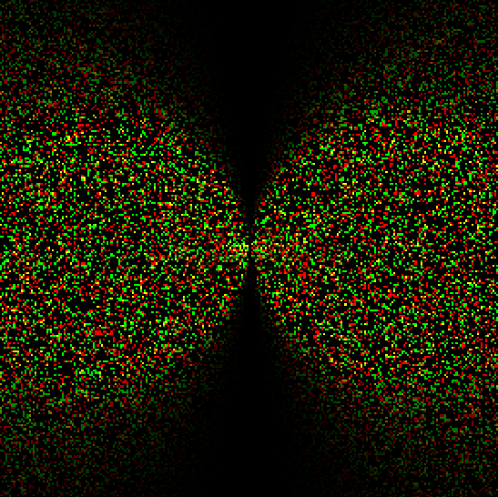
You can notice how the dot product between the normalized wave vector and the normalized wind direction is used to give more amplitude to waves in the direction of the wind, and less amplitude to waves in the orthogonal direction. This gives us the following 256x256 texture:
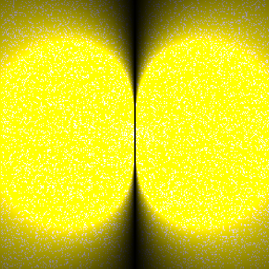
Here the origin is at the center of the texture, the distance to the origin gives us the frequency of the wave, and the angle gives us the direction of the wave. The value of the pixel then gives us the amplitude of the wave at that frequency and direction.
The color yellow is caused by using only the red and green channels of the texture (our spectrum is complex so we need a channel for the real part and a channel for the imaginary part).
But the real and imaginary parts are currently identical and oceanographic data shows waves have an inherent randomness to them. If we only use this spectrum, we will get many regularities in the ocean surface, and not get the realistic look we are aiming for.
The solution is to multiply our spectrum by some random numbers, like a complex gaussian noise with mean 0 and variance 1. Here is an example of gaussian noise texture:
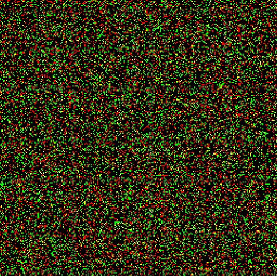
Each pixel is assigned a gaussian random number for the red channel, and another for the green channel. The blue channel is not used again.
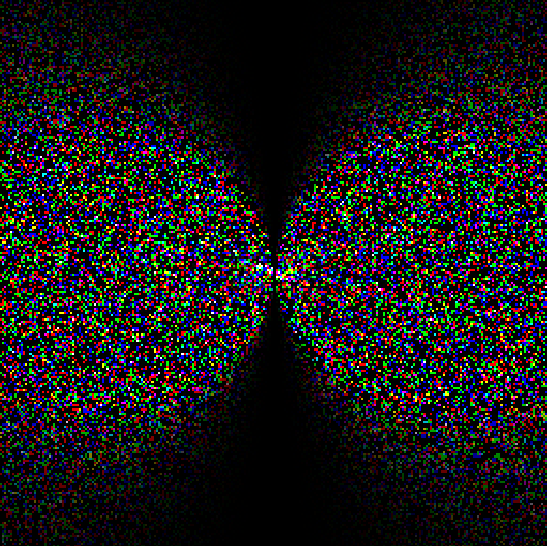
Now we take the product of the two:
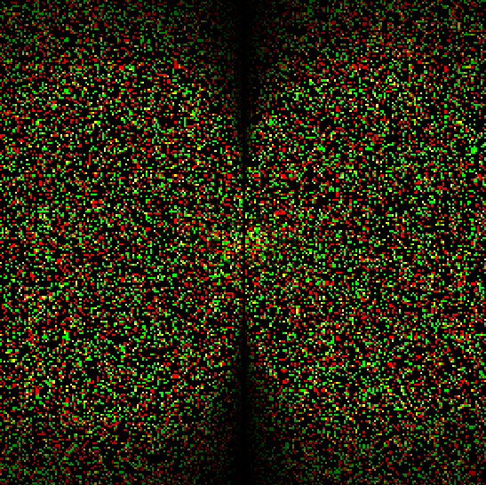
We can also increase the influence of the wind by raising the dot product between the wave vector and the wind direction to a greater power. For a 6th power, we get the following spectrum:
We can see clearly that waves with an orthogonal direction to the wind have a much lower amplitude than waves in the direction of the wind.
How to make it move?
This spectrum is all well and good, but we expect the ocean to move during the simulation: the wave amplitude and phases will change over time. The good thing is that from our initial spectrum, we can compute the spectrum of the ocean at any point in time, without having to care about what happens in between.
The formula to do that is given in Tessendorf’s paper and is as follows:
$$ \tilde{h}(k, t) = \tilde{h}(k, 0) \exp(i \omega(k) t) + \tilde{h}(-k, 0)^* \exp(-i \omega(k) t) $$
So we will need to use the conjugate of the initial spectrum to compute the spectrum at time t. As the conjugate is also a complex number, I chose to precompute the conjugates and store them on the same texture as the initial spectrum built earlier. As a texture has 4 channels, we can indeed store two complex numbers in one pixel.
Here is the result with the conjugate:
The blue shade is the real part of the conjugate, and the imaginary part is stored in the alpha channel which we cannot view here.
Note that the initial spectrum is only computed once, so you are not obligated to use a compute shader as it has no impact on the performance of the simulation.
The first bottleneck is the time-dependent spectrum computation. If the spectrum has a resolution of 512x512, it already requires 262144 complex multiplications with calls to trigonometry functions for the exponentials, each frame.
Therefore, this part must take place in a compute shader, or at least in a fragment shader.
Here is an animation of the time-dependent spectrum:
Computing the Inverse FFT
Our ocean surface is now well represented in the frequency space, but we need to go back to the spatial domain to render it. This is done by computing the Inverse FFT of the spectrum.
For small spectrum resolutions, you can probably get away with a CPU-side FFT using multithreading, but for larger resolutions, you will need to use compute shaders.
The GPU implementation of the FFT algorithm is quite complex, and you will probably want to use a library like GLFFT if you are implementing it in C++.
For WebGPU, I reused Popov72’s implementation of the FFT algorithm in TypeScript.
Now if we run the FFT on the spectrum, we get the following heightmap:
We have 2 colors here, red for the real part and green for the imaginary part. The actual height we are interested in is only the real part, but the imaginary part is also computed by the FFT algorithm.
As the values are not normalized, we don’t get to see a lot of details, but we can see something that looks like waves.
If we directly use this heightmap to deform a plane, we won’t see a realistic ocean:
This is because we are still missing the surface normals to compute the lighting. Fortunately, Tessendorf’s paper also derives the formula for the gradient of the waves, which we can use to compute the normals.
Computing the Normals
In order to compute the height of the waves, we took the IFFT of h(k, t), the time dependent spectrum. To compute the gradient, we will now perform as well the IFFT of i*k*h(k, t), where i is the imaginary unit and k is the wave vector.
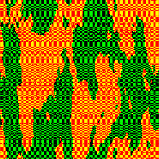
The expression is very similar, thus we can compute it at the same time as the time-dependent spectrum, getting this result:
After IFFT, we get this:
We clearly see the pattern of waves in the gradient map. The red channel is the x component of the gradient, and the green channel is the z component.
You may notice the visual artifacts in the corners of the gradient map. This is likely caused by the Phillips Spectrum, choosing another spectrum such as JONSWAP could help reduce these artifacts. They also disappear with time, so starting the simulation at t=60s is also a solution.
Choosing L=10m and a texture size of 256x256 with a simple Phong lighting model gives the following result:
We are getting there! But now we will take some time to make it look even better.
Shading
Skybox
First of all, water does not exist in a vacuum. Every ocean shot on camera also features a nice sky with a sun and sometimes clouds. We can simulate this by using a skybox: a cube with a texture of the sky on each face that will be rendered behind the water. BabylonJS has a nice asset library with beautiful skyboxes, so I chose tropical sunny day.
It’s already looking better:
With a sky so bright, our ocean looks very out of place, and that’s because the ocean must reflect the sky!
Fresnel Reflection
The fraction of light reflected by a surface depends on the angle between the surface normal and the view direction. This is called the Fresnel effect. You can find general formulas online that depend on the index of refraction of each medium, but for our purposes we will only use the water’s version:
$$ fresnel = 0.02 + 0.98 (1.0 - \theta_i)^5; $$
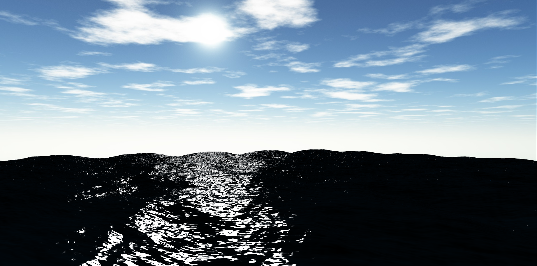
Using this formula to interpolate between the color of the ocean and the reflected color of the sky, we get the following result:
Specular
You might not be getting the nice white highlights on the waves that you can see on my screenshot. This is because I chose specific ranges for the exponent and the intensity of the specular highlights. I took them from afl_ext’s shader: 720 for the exponent and 210 for the intensity. You can tweak these values to your liking.
Transparency
Water is also transparent, and the deeper the water, the more opaque it becomes. To simulate transparency, we must first render the scene without the water (this will be our background image), then render the water on top of it with a transparency factor.
In BabylonJS, you can use a RenderTargetTexture to render the scene and then change the renderList to include all meshes except the water planes.
We must now sample this background image from the water shader. In the vertex shader we already compute the clip position of our vertices by multiplying their local position by the world matrix, then the view matrix and finally the projection matrix.
We can pass it to the fragment shader using a varying variable. As the clip position is in homogeneous coordinates, we must divide it by its w component to get the screen position between -1 and 1 in the x and y components.
Texture coordinates in GLSL are between 0 and 1, so we can remap the range to get the screen coordinates of each fragment of the water plane. We can then sample the background image at this position.
Choppy Waves
The waves are looking quite good now, but you may notice we don’t see sharp peaks on the waves, they look too round.
The issue is that for now we only translate our vertices vertically, but in reality the waves should also move horizontally, combining to create a circular motion.
Once again, Tessendorf’s paper comes to the rescue with nice mathematical derivations to achieve the choppy waves effect.
$$ D(x, t) = \sum_{k} -i \frac{k}{|k|} \tilde{h}(k, t) \exp(i k \cdot x) $$
As often in this project, the solution is to compute more IFFTs, and we will do just that for the horizontal displacement.
In the same compute shader as we compute the time-dependent spectrum, we will write a new texture which will hold these values:
$$ -i \frac{k}{|k|} \tilde{h}(k, t) $$
This is really similar to the gradient computation, we just added a multiplication by the normalized wave vector.
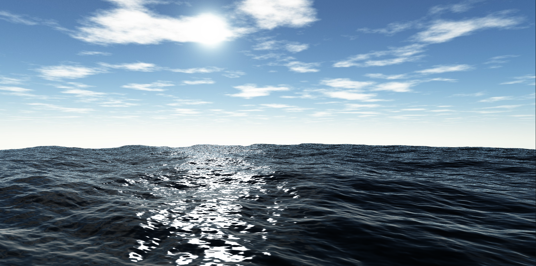
We can then plug the result of the FFT in our vertex shader to displace the vertices horizontally, giving us the following result:
This looks really nice! One extension now could be to use the gradient of the displacement to compute the foam using the Jacobian, but I won’t cover it in this post.
What I want now is to wrap it on a sphere!
A bit of fog
It can also be nice to add some fog on the horizon to blur the separation between the water and the sky. Fog is usually computed with an exponential decay function of the depth of the scene. The issue is that this gives an omnidirectional fog, while we want the fog to be only on the horizon, so that we can still see the sky when looking up.
We can do that by adding a multiplier to the fog factor that depends on the angle between the view direction and the horizon:
$$ fog = 1.0 - \exp(-\text{depth}^2 \times \text{fogDensity}^2) \times (1.0 - \cos(\theta))^4 $$
This gives a more atmospheric look to the scene:
Wrapping on a Sphere
One of the nicest features of the discrete Fourier Transform is that the resulting ocean tiles are seamless. This means that if you put two tiles next to each other, the waves will match perfectly, and you can tile them indefinitely:
This is a great feature for texture mapping a flat terrain for example. But as soon as your plane is not completely flat, the mapping will warp the textures in weird ways.
We are not exactly doing texture mapping, but all of our ocean data is stored in textures that are used to deform the vertices of our plane, so we will have the same issue.
One solution to avoid those warping artifacts on non-flat terrain is called “tri-planar mapping”. The idea is to project the texture on the terrain from 3 different directions and blend the results:
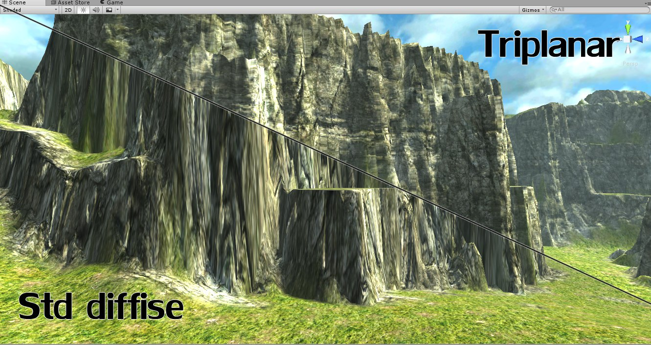
Triplanar Terrain Shaders from https://forum.unity.com/threads/free-triplanar-terrain-shaders.367992/
If you want to know more about it, I recommend Catlike Coding’s tutorial.
Tri-planar mapping is very versatile and can be used for more than 2D terrain. It can also be used to map a tillable texture on a any kind of geometry with defined normals and positions. This includes spheres among other things (like cubes, donuts, the only limit is your imagination).
To achieve this, we need to go in our vertex shader and change the sample coordinates for our height-map, gradient-map and displacement-map. Instead of using the uv coordinates, we will use the position of the vertices in sphere space to sample each texture 3 times and blend the results using the normals of the vertices.
Instead of changing the y component of the vertex position, we will translate it along the normal of the sphere by the desired amount.
One issue that remains is the computation of the normal vector to the ocean as well as the displacement. We cannot rely on shifting the vertex along the x and z coordinates, we want to move the vertex in the tangent plane to the sphere.
In order to achieve this, we will need two orthogonal tangent vectors to the sphere at the vertex position: the tangent and the bitangent. We can compute them using the spherical coordinates of the vertex position:
$$ \vec{t_1} = (-sin(\phi), 0, cos(\phi)) $$ $$ \vec{t_2} = (cos(\theta)cos(\phi), -sin(\theta), cos(\theta)sin(\phi)) $$ $$ \text{Where } \theta \text{ is the longitude and } \phi \text{ is the latitude} $$
Now we can displace the vertices along the two tangents for the displacement, and we can express the gradient of the waves in terms of those two tangents as well.
Once all of this is done, we get our water ball:
The next step will be to integrate it into Cosmos Journeyer, and I will keep you updated on the progress!
Conclusion
20 years after Tessendorf’s paper, the FFT ocean simulation is still a great way to generate realistic oceans. With the power of modern GPUs, the FFT has become really cheap to compute, and we can now simulate detailed oceans in real-time.
There are many extensions possible to this project: foam generation, refraction, underwater caustics, more spectrums like JONSWAP, etc. I didn’t have the time to implement them all, but it was nonetheless a great and fun learning experience.
All the source code for this project is available here under the MIT license if you want to use it in your own projects.
I hope this post was helpful to you, and that you will be able to use this technique in your own projects. If you have any questions, feel free to ask them in the comments!