I have been making a soft body simulation in C++ for my IMA904/IG3DA class at Telecom Paris, and I thought I could share my project report here! This one is quite light on the implementation details and is more focused on the high level ideas.
I added many example videos from the original report to make it more interesting to read!
Anyway, here is what you can expect from this article:
The full source code is as always available under a public license on GitHub (see the link at the end of the article).
I hope you will enjoy it!
Abstract
Soft bodies are a notoriously challenging field of computer simulations. Making it real-time brings additional constraints (very funny PBD joke haha), requiring trade offs between performance and accuracy. Since more than a decade, the Position Based Dynamics (PBD) family of simulation methods have been very successful at making good looking soft bodies in real-time. From the original PBD [Tsai 2017] method came improvements to stability and convergence speed with Hierarchical Position Based Dynamics (HPBD) [Müller 2008] and eXtended Position Based Dynamics (XPBD) [Macklin et al. 2016].
Although my initial goal was to implement HPBD, combining it with XPBD felt very natural and yield powerful results.
Introduction to PBD
Just for starters, I will briefly describe the core concepts of PBD, and how it differs from classic rigid body simulations.
Particles vs Rigid bodies
In rigid body physics, the object is often represented as one single entity. This is not enough to simulate soft bodies, as we need to make local changes to the object (stretching, bending…).
In PBD, every object is represented by a set of particles (usually the vertices of the triangle mesh), allowing the PBD solver to manipulate them separately, creating deformations.
Forces vs Constraints
In rigid body physics, forces are simulated to make the object move in a realistic way, with some variations including impulses to modify the velocity of the object in the case of collisions.
PBD uses a totally different approach. Instead of simulating forces, PBD directly modifies the positions of the particles! (Hence Position in Position based dynamics).
How does it work? The particles are linked together by constraints, that must be satisfied at every frame. Constraints can be of many types: 2 particles must keep the same distance, 4 particles must keep a constant volume, a particle must stay at a fixed position, etc.
If you have a flat piece of cloth for example, you can create distance constraints between every pair of neighboring vertices, and then add a fixed constraint to the 4 corners of the cloth to make a deformable kind of trampoline.
The constraints can be hard, meaning for the distance constraint that the distance between the 2 particles must be exactly the same as the initial distance, or soft, meaning that the distance can vary a little bit. The stiffness of the constraint will determine how much the distance can vary.
Here is a visual example of decreasing the stiffness of the distance and bending constraints:
For the piece of cloth example, we would want the distance constraints to be soft, and the fixed constraints to be hard, so that the cloth can stretch, while the corners stay in place.
At every frame, the PBD solver will take the constraints of all particles and move the particles in order to satisfy the constraints!
To perform collisions, constraints are created every frame between the particles from one body and the triangles (3 particles) of another body, pulling them apart to prevent penetration.
If you want to read the paper to have a more detailed explanation, you can get the paper here [Müller et al. 2007].
Motivation
Even though Position Based Dynamics comes in different flavors, they are all based on the same fundamental concepts. Each object is represented as a set of particles, whose positions change based on constraints (distance, volume, collision…) instead of simulating forces like in classic rigid body simulations.
Classic PBD is not perfect, and different extensions have been proposed to mitigate its shortcomings. One of the issues is the convergence speed. In order to achieve a realistic looking result, multiple constraint solving steps are required.
Local position changes propagates slowly to other parts of the same body as the number of vertices, and thus constraints grows. One solution is then to take a shortcut through the constraints by using coarser resolutions of the same object. The coarsest levels of the mesh will allow fast propagation of movement through the entire object, while the finer constraints will take care of the finer details. This hierarchy of resolutions (hence HPBD) makes the system converge in less steps, thus we can make the simulation faster.
Even though the simulation is faster, it can still become unstable in the context of collisions between 2 dynamic soft bodies. Extended Position Based Dynamics (XPBD) is a modification of the Gauss-Seidel solver that confers unconditional stability and faster convergence speed to the simulation. It is entirely compatible with HPBD and is part of my final implementation.
Mesh Decimation
Triangulation
The first step toward the multi-grid solver is to create the subgrids for each soft body. Each body is composed of vertices, linked together by triangles. The goal is to take the initial vertex data, and output a new batch of data with fewer vertices, and fewer triangles that have similar area between each other. The HPBD paper proposes the general reduction algorithm to perform the decimation and its implementation yield good results for complex meshes such as the Stanford Bunny.
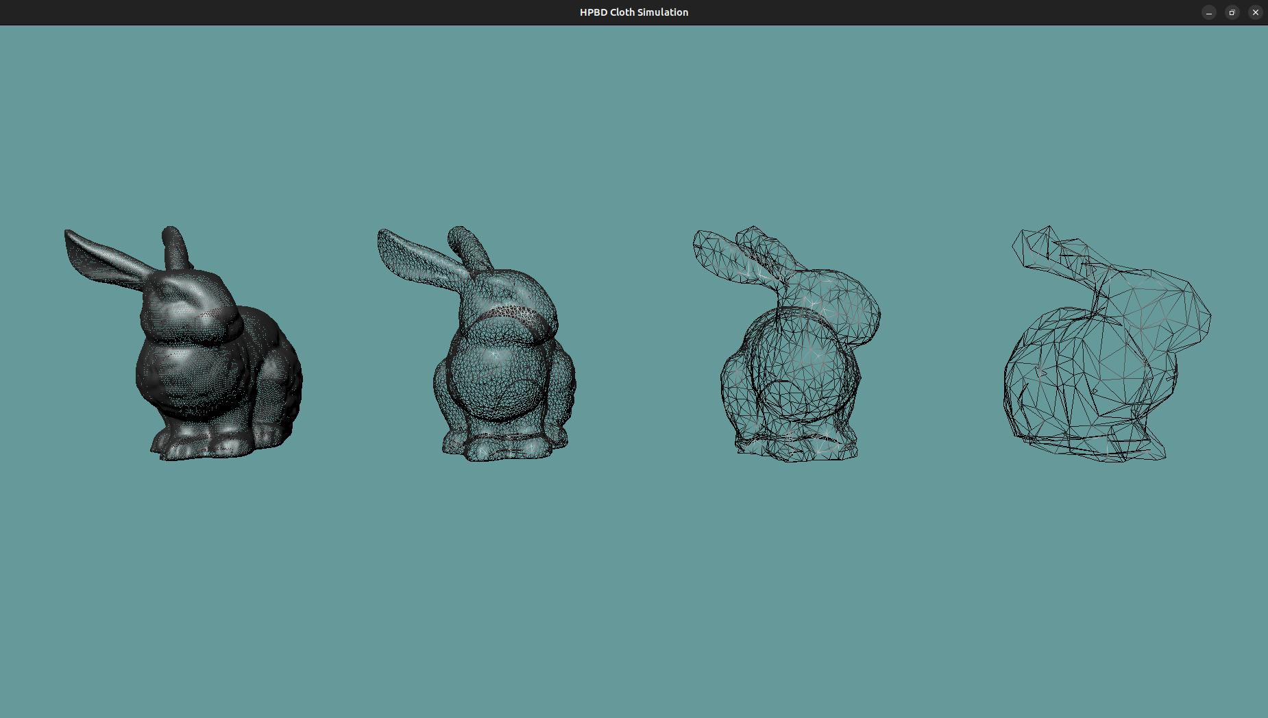
One limitation is that sometimes the general reduction algorithm outputs a non-manifold mesh, which causes issues when deciding whether or not to create a global volume constraint (more on that later).
Constraints
The next step is then to bring our constraints to the coarser levels of the geometry so that we can propagate the error faster. The paper describes the procedure and is quite easy to understand: copy all the constraints from the finer level to the coarser level.
As not all particles are present in the coarser level, we replace the fine particles by a coarse neighbor (i use the closest). This yields a new set of constraints that we can filter to remove duplicates or outliers.
Once the hierarchy is built, we don’t have to change it as long as the geometry of the mesh is unchanged (i.e no tearing). It will also be useful for the collision part, stay tuned for that!
Implemented Constraints
PBD is all about the constraints you can simulate. The more diverse the constraints, the more complex scenarios can be simulated. However, deriving the gradients of the constraints is a lot of math, thankfully the papers provided good starting points and I could find the gradient formulas on internet.
If you want a taste of the gradient derivation, you can check out blackedout01’s awesome video featuring the gradient of the dihedral constraint:
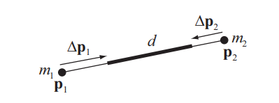
Distance Constraint
The most fundamental constraint is the distance constraint. Make it rigid and you have a rigid body, make it soft and you can already simulate flat cloth pieces. This one has all the math already done in the original PBD paper so it didn’t cause any issue.
Fixed Constraint
Once the distance constraint is implemented, the fixed constraint is just a small specialization. Instead of specifying the distance between 2 particles, we only need to specify one particle and a target position. We can then make it a hard constraint (stiffness=1 for PBD, compliance=0 for XPBD). Some methods advise to also set the mass of the particle to 0, so that it won’t move at all in the simulation. I found it was not necessary as the fixed particles stayed in place. Moreover, not doing that allows to increase the compliance of the constraint while simulating which gives more freedom to the user.
Bending Constraints
Dihedral Bending Constraint
Although we studied the dihedral constraint in class, I did not implement it at first.
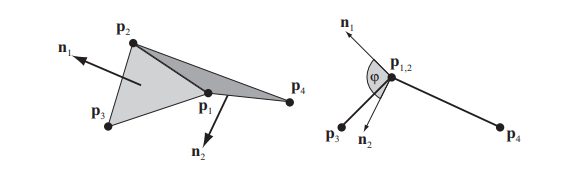
It’s main advantage is that by targeting the angle between the triangles, the constraint becomes independent from stretching created by classic distance constraint.
The main drawbacks are that the gradient derivation is horrendous, and is quite slow and unstable because of acos function calls. You will get a lot of NaNs if you are not careful!
I ended up implementing it anyway as an attempt to solve the collision issues that I will cover later. It did not change anything, but it is still a nice addition to the constraint bestiary.
Fast Bending Constraint
My favorite bending constraint is the fast bending constraint. It is also the easier one to implement as it only involves a distance constraints between opposed vertices of neighboring triangles.
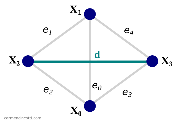
I came across it on Carmen Cincotti’s website while looking for information on the dihedral constraint. Although it is not independent of stretching, it is much faster which makes it worth it to reach real-time speed.
Volume Constraints
Tetrahedral Volume Constraint
The first volume constraint I implemented was the Tetrahedral Volume Constraint. As in the name, it constrains the position of 4 particles to keep a constant volume of the formed tetrahedron.
I considered using it in conjunction with Tetrahedral meshes, but it seemed unnecessary complex compared to the Global Volume Constraint.
Global Volume Constraint.
The next one is the global volume constraint (so surprising I know). It takes all the particles of a given mesh, and preserve its volume over time. The formula for this one is beautifully simple given the number of particles involved. (It doesn’t mean it worked on the first try of course!) It is one of the most important constraints that makes the biggest visual difference. While distance and bending constraints can already conserve some volume when using an important stiffness, it always looks like the object is about to collapse on itself. The global volume constraint allows for a funnier result with more bouncing and you can also simulate over-pressure just like in the original paper.
The over-pressure and under-pressure tends to make the object rotate on itself (like with a ghost force). I found a good explanation in this video [blackedout01 2023]. Basically it is linked to the fact the constraint are always solved in the same order, thus the systematic error will never be cancelled out.
One way to fix this is to solve the constraints in a random order. The issue is that HPBD forces the order of the solver in some sense. The coarser levels must be solved before the coarser ones. Maybe randomizing the solving order inside each hierarchy level could improve it a little bit, but I did not try it.
Collision Constraint
Last but certainly not least is the collision constraint! It is always presented as something easy in the papers, with a very hand wavy description and I had to fail a lot before getting a nice and believable result.
Warm up: ground collisions.
I first started with ground collisions. It is a bit of a hack, but you have to start somewhere. Basically it just involved clamping particle positions y coordinate to be always greater or equal to 0. It worked really well, and I was confident the rest would come into place nicely. I was wrong.
True collision pipeline.
The PBD papers proposes a simple collision constraint that involves a particle, and 3 other particles forming a triangle. The constraint keeps the first particle on one side of the triangle, preventing penetration.
The constraint implementation in itself was not very difficult, although I did not get the gradient right at first, and I had to find Sammy Ramasimanana’s (a friend from the IGD master!) last year implementation of XPBD [Rasamimanana 2023] to find where my mistake was.
But fixing the gradient was far from enough! Here are some of the bugs that still destroyed my simulations:
Fixing the collision issues
I spent an entire week fixing the collisions in my simulations so I have plenty to report on that.
The first thing is about the constraint itself. It is presented as a particle triangle constraint while in reality it is a particle to infinite plane constraint!
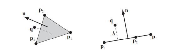
The constraint keeps the particle on one side of the infinite plane that contains the triangle, which can become awful when you have a lot of different triangles! (With so many infinite planes with random orientations, you will always be on the wrong side!).
Therefore the challenge becomes to find very precisely the pairs of particles/triangles so that we don’t get a distant triangle interacting in a completely weird way with some particles of another object.
Broad phase
Last year, I made a small rigid-body engine.
It used a 2 phase system: first, a broad phase to find pairs of neighboring bodies, and then a narrow phase where the geometry is involved, is used to solve the actual collisions.
In the same way as last year, I added an Axis-Aligned Bounding Box (AABB) to every physics body of my scene.
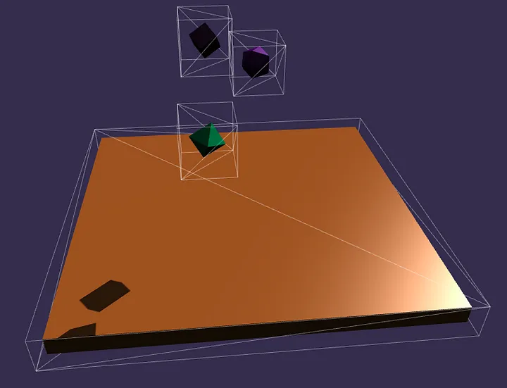
In the broad phase, I check all AABB against each other (sorry for the O(n^2), I didn’t have the time to back port my spatial hash grid to C++).
One of the nice properties of AABBs is that the intersection of two AABBs is another AABB. Therefore every AABB to AABB contact will give us another AABB to work with in the narrow phase. By only working inside the AABB intersection, we can already get rid of many particles and triangles.
Narrow phase
Now for each body, I find all the particles inside the intersection AABB, as well as all the triangles intersecting it. At first, I created a collision constraint for every particle/triangle pair of this intersection. This was not good enough and created many errors.
I tried changing the bending constraint and even ended up implementing XPBD as a way to make the simulation more stable. While it definitely helped a bit, it was not the real issue. I had to get better as selecting particle/triangle pairs.
The next thing I implemented was to shoot a ray from the center of mass of the object to the surface particle and then checking the intersection of this ray with the faces of the other body:
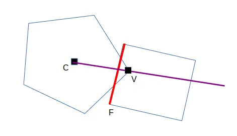
This already fixed the instabilities I had, but using the center of mass is not perfect when the mesh is not perfectly convex (think of a torus, the center of mass is not inside the object so a ray coming from the center of mass to a surface vertex could intersect a triangle from another body while no collision is happening).
A better solution was then to shoot a ray from the particle itself in the direction of the particle normal. It made the collision with the flat cloth better as well because the ray from the center of mass to the particle would actually be completely wrong as well in the case of a flat piece of clothing.
Finally we can get clean, 2-way collisions between dynamic soft bodies!
Surface friction
Now that the collision finally works, I want to fix the cringe sliding effect that the mesh tend to have while sitting on the ground. Objects in real life have surface friction that prevent this.
Here is an example of cube sliding like they were on ice:
My solution for that is a bit hacky in my opinion but it works. Basically at the end of a simulation sub-step, I check every particles of every object and check if there is a collision constraint that utilizes it.
If that is the case, I compute the normal of the associated triangle.
Then I can take the current particle’s velocity and subtract the normal component (using a dot product) to get the tangential velocity. The next step is to scale it using a lower than one factor to mimic friction.
I then add back this dampened tangential velocity to the normal component of the particle velocity, and the result is quite convincing!
It stopped the sliding effect. A possible extension could be to define the friction coefficient per body, and not globally like it is the case currently.
Performance improvements
HPBD accelerated collisions
HPBD already increases the speed of convergence of the solver, but I thought I could take advantage of the hierarchy to speed up collisions. In fact, when a sphere is colliding with the flat piece of clothing, we don’t need to check all the many triangles of the cloth. We only need an approximation of its shape to get a convincing result. Thankfully we already built a hierarchy with approximations of the original mesh.

Therefore, I only needed to check the collisions against the hierarchy level I wanted. For now it is user defined and highly depends on the geometry of the clothing, but automatic estimation of the right level to use can probably be found. Using the right level of collision allows for a nice speed up for complex meshes.
In this video, the framerate goes from 30 fps on using the entire geometry to 60 fps using the first level of the hierarchy of the cloth:
Making the most of XPBD
Reflecting on the whole project, implementing XPBD was probably not necessary to make the collisions work properly. So how can we make the most of it? XPBD is a modification of the PBD solver by changing solver iterations by solver sub-steps: the collisions are only solved once per subset instead of multiple time per step.
To upgrade from simple PBD to XPBD, I found the video from Matthias Müller, one of the original author of the paper, to be very straightforward and helpful:
This is a surprisingly simple and yet powerful change that make the convergence rate of PBD much faster. One of the original author even describes it as rendering obsolete the old HPBD method. While XPBD alone is better than HPBD alone, I think the combination of both can be powerful (just the collision performance improvement is huge, and can’t be overlooked).
As XPBD increases again the convergence rate of the solver, I was able to half again the number of solver sub-steps, only performing 4 solver steps every frame.
All of this taken together allowed for real-time frame-rate of complex soft bodies (60 fps for an ico-sphere with a 32x32 flat piece of cloth).
CPU PICKING
The last big feature I implemented for this project is CPU picking. I was heavily inspired by this awesome video from blackedout01:
It was very helpful for validating my implementation and featured the awesome ability to grab an object with the mouse and move it around (and make it wobble).
Getting a ray from the mouse
The CPU picking is done by performing a ray-cast from the camera. The first step is then to get a ray from the camera, going through the mouse clip position.
I based my implementation on this post from stackoverflow that was very helpful.
Basically, we convert the mouse position to a [0;1] 2D vector by dividing its coordinates by the dimensions of the window.
We then create the clip space position by converting these coordinates to the [-1;1] range, and specifying 0 and 1 for the z and w homogeneous coordinates.
From this clip position, we can then use the inverse of the camera projection matrix to get the view space position of the mouse in the
scene.
We then can get the world position by using the inverse of the camera view matrix.
From this world position and the camera’s world position we indeed get a ray!
Shooting the ray
Now we can take advantage of our AABBs for the picking as well. We shoot the mouse ray and check the intersections with the different AABBs. We then take the closest hit object and find out if a triangle is intersecting with the ray.
If it is not the case, we check the second closest object and so on.
Once we have the id of the intersected triangle, we can start thinking about dragging our objects.
Body dragging
In the video, distance constraints are created between the mouse position and the particles of the intersected triangle. When the mouse move, the particles will follow until mouse release using the solver.
While I think using the solver for this is a really good idea, my code architecture did not really support removing constraints on the fly beyond the collision constraints.
I decided to use a different approach. When I get an intersection with a triangle, I compute the barycenter by simply averaging the particle’s positions. Then, I can compute the difference with the mouse intersection point to get a translation vector. The next step is then to translate the whole body using this translation vector.
This is already good and useful, but we won’t get the wobbling effect just like that. The trick I used is to translate the body particles by a fraction of the mouse translation: closer particles get a stronger pull while distant particles will lag behind. In more technical terms, I use an inverse distance kernel to translate my particles.
I also tried using the squared distance, but the result was disappointing and less fun that using the inverse distance. The last issue I had to address is that the object could tend to come toward the camera because of how the translation vector is calculated. This was easily solved by storing the initial depth of the intersection and then using it while dragging to ensure constant distance to the camera.
Conclusion
In the end, we have a really solid soft body simulation that runs very fast with interacting soft bodies. Merging HPBD with XPBD resulted in a very powerful combination that enabled faster collisions and greater convergence speed overall.
There are still many avenues of improvements for future work! Choosing the right level of hierarchy for the collisions could be automated using some kind of vertex density threshold. The solver could also be parallelized using multi-threading or even a compute shader, which would make an enormous difference in performance!
Another possible area of improvement that actually has some basic implementation in my code is cloth tearing by discarding the edges that violate the distance constraints by a too large amount. I already got the edge removing process working, but sadly I did not have time to make the system to remove dynamically the distance constraints:
Moreover, more constraints could be implemented such as the Isometric Bending Constraint, and the very hard Self Collision Constraint.
I only experimented with a uniform gravity field, but it would be easy to try some spherical gravity just like with Avalanche last year.
It would also be desirable to back port the spatial hash grid from Avalanche to make the collision narrow phase much faster.
As I discussed earlier, friction could be defined per body, and a restitution coefficient could also be added, although I am not sure what would be the best way to implement it. Maybe a simple scaling factor on the normal component of the particle velocity would be enough just like for friction.
The entire source code is available on GitHub under a public domain license for anyone to use and improve. It was a really fun project and I learned a lot while implementing it.
Acknowledgments
I would like to thank Dr. Kiwon Um of Telecom Paris for being an awesome computer graphics teacher. I enjoyed a lot learning from your classes during my 2 years of IGD master.
References
blackedout01. 2023. Writing a soft body cube in C/C++ using XPBD | Devlog Episode 2. (2023). https://www.youtube.com/watch?v=J1nojsTnw_M&t=287s
Carmen Cincotti. 2022. The Most Performant Bending Constraint | XPBD. (2022). https://carmencincotti.com/2022-09-05/the-most-performant-bending-constraint-of-xpbd/
Miles Macklin, Matthias Müller, and Nuttapong Chentanez. 2016. XPBD: PositionBased Simulation of Compliant Constrained Dynamics. DOI: https://doi.org/10.1145/2994258.2994272
Matthias Müller. 2008. Hierarchical Position Based Dynamics., Vol. 8. 1–10. DOI: https://doi.org/10.2312/PE/vriphys/vriphys08/001-010
Barthélemy Paléologue. 2023. Avalanche Rigidbody engine. (2023). https://github.com/BarthPaleologue/Avalanche
Barthélemy Paléologue. 2024. Feather Rendering Engine. (2024). https://github.com/BarthPaleologue/feather
Sammy Rasamimanana. 2023. XPBD: Position-based simulation of compliant constrained dynamics. (2023). https://github.com/LemillionX/IMA904_XPBD/tree/master
Matthias Müller, Bruno Heidelberger, Marcus Hennix, John Ratcliff. 2007. Position based dynamics. DOI: https://doi.org/10.1016/j.jvcir.2007.01.005